4. Analysis of the Parallel Performance for the Test Problem
In all F90 and Python implementations of this work, the GNU 4.8.5 compiler set and the OpenMPI 4.0.1 library were employed, with the -O3 optimization flag. In the case of F90 implementations, the version compiled with the Intel 19.1.2 and Intel MPI 19.1.2 library was also tested, however the performance results were similar and, therefore, only GNU gfortran with OpenMPI is shown in the rest of this work. It is important to note that only one Bull Sequana X node was available and, therefore, in general, tests of one and several nodes were performed using Sequana B710 nodes.
4.1. Comments on the Performance of the CPU-executed Implementations
Processing times (the numbers 1, 4, 9, ... , 81 are the MPI processes)
| Serial | 1 | 4 | 9 | 16 | 36 | 49 | 64 | 81 | |
|---|---|---|---|---|---|---|---|---|---|
| F90 | 19.25 | 21.91 | 7.34 | 6.15 | 4.68 | 2.13 | 1.89 | 1.23 | 1.69 |
| F2Py | 18.94 | 23.60 | 7.45 | 6.17 | 4.62 | 2.15 | 1.63 | 1.27 | 1.01 |
| Cython | 23.97 | 23.98 | 7.46 | 6.29 | 4.69 | 2.23 | 1.67 | 1.31 | 2.06 |
| Numba | 30.48 | 30.53 | 8.18 | 6.33 | 5.86 | 3.22 | 2.68 | 1.79 | 2.07 |
| Python | 212.43 | 227.19 | 64.74 | 44.78 | 33.46 | 15.21 | 10.43 | 7.85 | 6.70 |
Speedup (the numbers 1, 4, 9, ... , 81 are the MPI processes)
| Serial | 1 | 4 | 9 | 16 | 36 | 49 | 64 | 81 | |
|---|---|---|---|---|---|---|---|---|---|
| F90 | 1.00 | 0.88 | 2.62 | 3.13 | 4.11 | 9.04 | 10.21 | 15.67 | 11.42 |
| F2Py | 1.02 | 0.82 | 2.58 | 3.12 | 4.16 | 8.96 | 11.83 | 15.14 | 19.03 |
| Cython | 0.80 | 0.80 | 2.58 | 3.06 | 4.10 | 8.64 | 11.55 | 14.74 | 9.36 |
| Numba | 0.63 | 0.63 | 2.35 | 3.04 | 3.29 | 5.98 | 7.19 | 10.75 | 9.32 |
| Python | 0.09 | 0.08 | 0.30 | 0.43 | 0.58 | 1.27 | 1.85 | 2.45 | 2.87 |
Parallel efficiency (the numbers 1, 4, 9, ... , 81 are the MPI processes)
| Serial | 1 | 4 | 9 | 16 | 36 | 49 | 64 | 81 | |
|---|---|---|---|---|---|---|---|---|---|
| F90 | 1.00 | 0.88 | 0.66 | 0.35 | 0.26 | 0.25 | 0.21 | 0.24 | 0.14 |
| F2Py | 1.02 | 0.82 | 0.65 | 0.35 | 0.26 | 0.25 | 0.24 | 0.24 | 0.23 |
| Cython | 0.80 | 0.80 | 0.65 | 0.34 | 0.26 | 0.24 | 0.24 | 0.23 | 0.12 |
| Numba | 0.63 | 0.63 | 0.59 | 0.34 | 0.21 | 0.17 | 0.15 | 0.17 | 0.12 |
| Python | 0.09 | 0.08 | 0.07 | 0.05 | 0.04 | 0.04 | 0.04 | 0.04 | 0.04 |
The Table 1 shows the processing times for the different implementations, in one or more Bull B710 nodes, for serial and MPI with 1, 4, 9, 16, 36, 49, 64 and 81 processes. These processes allow for perfect square subdomains (as explained in section 2) in the implementation performed.
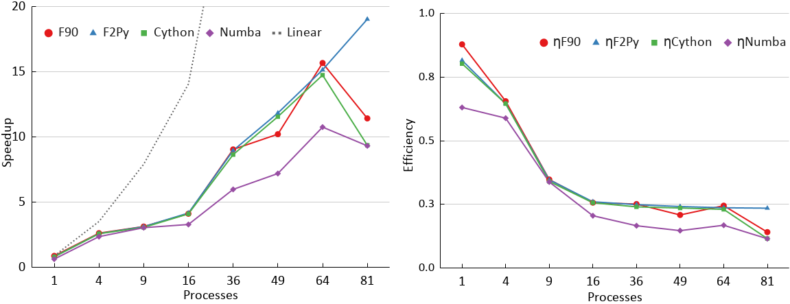
The Figure 2 shows the corresponding speedups calculated using the F90 serial time as a reference. In general, F90 and F2Py achieved the best performances and are followed by Cython and Numba, with Python well behind. F2Py requires few changes to the original F90 code, while Cython and Numba requires minor changes to the Python code. However, Numba's performance was comparable, from 4 to 36 processes. The low performance of Python versions shows the convenience of using implementations like F2Py, Cython, or even Numba. As can be seen, the parallel scalability is poor, since the test problem algorithm updates all points of the grid at each time step, thus requiring the exchange of boundary temperatures between neighboring subdomains, in order to update the phantom zones corresponding, requiring a lot of communication between processes, which leaves the parallel efficiency below 40% for processes of 9 MPI or more. It can be seen that for up to 36 MPI processes, running on two Bull B710 nodes, all implementations performed similarly, except for standard Python. In the case of 81 MPI processes, which requires 4 computer nodes, the performance of the implementations has dropped significantly compared to 64 MPI processes, which requires 3 nodes. It is intended, as a future work, to investigate the reason for the performance differences between the different implementations. Besides these CPU-executed implementations, the next section briefly shows the use of a GPU-executed implementation.
4.2. Processing Performance of the Numba-GPU Implementation
Numba-GPU implementation was made as an example, in order to make a very rough comparison between the performance of CPU and GPU implementations. It should not be used to draw conclusions, as such a comparison would require an extensive number of tests. This section aims to compare the performance on a single node, of: (i) implementation of a single Numba-GPU process performed on a Bull B715 node, or Bull Sequana-X node; (ii) single and serial F90 process implementations running on one or more processor cores of the Bull B715 node or Bull Sequana-X node. Note that Bull Sequana-X is a very up-to-date SDumont node, with the latest processors and GPUs. The Numba-GPU implementation was tested on a Bull B715 node using a single core, and the Tesla K40 GPU runs at 22.28 s, close to the execution time of the F90 serial implementation. The same Numba-GPU implementation performed on a Bull Sequana-X node using a single core and a single Volta V100 GPU, was performed in just 8.02 s, slightly more than most parallel implementations running with 4 MPI processes in the Bull B715 node. The implementation of the Numba-GPU required more modifications compared to the standard Python serial code than the others. The loop was encapsulated in a function with a Numba decorator to be executed on a single GPU using just-in-time (JIT) compilation. These execution times correspond to blocks of $ 8 \times 8 $ threads in the case of the GPU V100 (node Bull Sequana-X), and blocks of $ 16 \times 16 $ threads in the case of the GPU K40 (node Bull B715). These block sizes have been optimized by trial and error. The multi-threaded single instruction (SIMT) paradigm models the execution of the GPU, with the problem domain mapped in a block grid composed of a series of threads. The blocks are then divided into warps, usually 32 threads, and executed by one of the streaming multiprocessors that make up the GPU. Numba-GPU uses a wrapper for the CUDA API in C language, providing access to most of its features.