2. The Five Point Stencil Test Problem
The adopted test problem is a known problem of heat transfer over a finite surface, modeled by the partial differential equation of Poisson. It models the normalized temperature distribution on a surface over a series of iterations that make up the simulation. As commonly used for numerical solutions, this equation is discretized in a finite grid and solved using a finite difference method. The specific algorithm requires the calculation of a 5-point stencil in the 2D domain grid [4] to update temperatures every step of the time. A uniform temperature field with a zero value is assumed on the surface and, typically, adiabatic or Dirichlet boundary conditions are assumed, the latter being assumed for this problem. Three constant rate heat sources were placed at localized grid points, each introducing an amount of unit heat in each time interval. The heat transfer simulation is modeled by a finite number of time steps, with all points on the grid being updated at each time step. The temperature distribution will be determined by the heat sources and the boundary conditions of Dirichlet, which implies zero temperature at the points of the boundary grid [7]. The 5-point stencil consists of updating a point on the grid by averaging the temperatures of yourself with the temperatures of your four neighbors, left-right and top-bottom in the grid. The temperature field $ U $ is defined on a discrete grid $ (x, y) $ with spatial resolutions $ \Delta x = \Delta y = h $. Thus, discretization maps the real Cartesian coordinates $ (x, y) $ to a discrete grid $ (i, j) $, with $ U_ {x, y} = U_ {i, j} \,, \, U_ { x + h, y} = U_ {i + 1, j} \, $ for the dimension $ x $ and similarly for the dimension $ y $. The 2D discretized Poisson equation with a 5-point stencil is expressed by the Equation
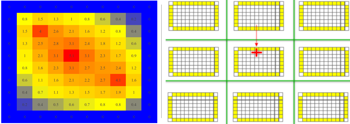
Considering the chosen test problem, an initial implementation of the algorithm proposed by Balaji [2] in the C language, was easily ported to F90. The discretized 2D domain of the heat transfer problem chosen as the test problem, showing 9 subdomains divided by green lines, with their grid points and phantom zones in yellow, is shown to the right of Figure 1, where the red cross denotes the 5-point stencil. The left side of Figure 1 shows the final temperature distribution over a finite surface after 500 iterations, exemplified by the grid $ 10 \times 10 $ and three arbitrarily chosen heat sources, shown as red cells, where the simulation only covers the inner grid $ 8 \times 8 $, and the initial zero temperature distribution is indicated in blue. This scheme requires splitting the original square domain into a perfect square number of square subdomains.